Alternating randomized least squares with leverage scores for CP Decomposition

>> Tensor Toolbox >> CP Decompositions >> CP-ARLS-LEV

The function cp_arls_lev computes an estimate of the best rank-R CP model of a tensor X using alternating randomized least-squares algorithm with leverage score sampling. The output CP model is a ktensor. The algorithm is designed to provide significant speed-ups on large sparse tensors. Here we demonstrate the speed-up we obtain on a tensor with 3.3 million non-zeros which can be run on a laptop. In the associated paper, CP-ARLS-LEV has been run on tensors of up to 4.7 billion non-zeros on which it yields a more than 12X speed-up as compared to cp_als.

CP-ARLS-LEV can also be run on dense tensors, and its performance is roughly equivalent to CP-ARLS. (CP-ARLS cannot be run on sparse tensors because it requires a mixing operation that destroys the sparsity of the tensor.)

The CP-ARLS-LEV method is described fully in the following reference:

B. W. Larsen and T. G. Kolda. Practical Leverage-Based Sampling for Low-Rank Tensor Decompositions. SIAM Journal on Matrix Analysis and Applications 43(3):1488-1517, 2022. https://doi.org/10.1137/21M1441754

Load in the Uber tensor
Running the CP-ARLS-LEV method with default parameters
Specifying how to compute the fit
Extracting and plotting the results
Specifying the number of samples
How to Select the Number of Samples
Comparing with CP-ALS
Running with estimated fit
Running with hybrid sampling
What is contained in the output info

Load in the Uber tensor

We will demonstrate how to run CP-ARLS-LEV using a sparse tensor constructed from Uber pickup data in New York City in 2014. The tensor has four modes - date of pickup, hour of pickup, latitude, longitude – and each entry correspond to the number of pickups that occured in that time and place. The tensor has 3.3 million nonzeros and can be found at https://gitlab.com/tensors/tensor_data_uber.

load uber
X = uber;
clear uber;
whos

sz = size(X);
d = ndims(X);

  Name        Size                          Bytes  Class       Attributes

  X         183x24x1140x1717            132380136  sptensor

Running the CP-ARLS-LEV method with default parameters

Running the method is essentially the same as using CP-ALS, feed the data tensor and the desired rank. Each iteration is printed as ExI where E is the epoch and I is the number of iterations per epoch. The default iterations per epoch is 5 (set by epoch) and the default maximum epochs is 50 (set by maxepochs). At the end of each epoch, we check convergence using an estimated fit baed on sampling elements of the tensor (this can be changed via truefit). Because this is a randomized method, we do not achieve strict decrease in the objective function. Instead, we look at the number of epochs without improvement (set by newi) and exit when this crosses the predefined tolerance (set by newitol), which defaults to 3. The method saves and outputs the best fit, which may not be the fit in the last epoch.

% Set up parameters for run:
R = 25; % Rank of the decomposition

% Run the algorithm:
rng("default"); % Set random seed for reproducibility
tic
M = cp_arls_lev(X,R);
time = toc;

Preprocessing Finished 

CP-ARLS with Leverage Score Sampling:

Tensor size: 183 x 24 x 1140 x 1717 (8596812960 total entries)
Sparse tensor: 3309490 (0.038%) Nonzeros and 8593503470 (99.96%) Zeros
Finding CP decomposition with R=25
Initialization: random (uniform)
Fit change tolerance: 1.00e-04
Epoch size: 5
Max epochs without improvement: 3
Max epochs overall: 50
Row samples per solve: 131072
No deterministic inclusion 
Fit based on: stratified with 132380 nonzero and 132380 zero samples
When to calculate true fit? never

Iter  1x5: f~ = 2.086947e-01 f-delta =  2e-01 time = 3.5s (fit time = 0.0s) newi = 0
Iter  2x5: f~ = 2.178264e-01 f-delta =  9e-03 time = 3.3s (fit time = 0.0s) newi = 0
Iter  3x5: f~ = 2.188760e-01 f-delta =  1e-03 time = 3.1s (fit time = 0.0s) newi = 0
Iter  4x5: f~ = 2.203693e-01 f-delta =  1e-03 time = 3.1s (fit time = 0.0s) newi = 0
Iter  5x5: f~ = 2.200585e-01 f-delta = -3e-04 time = 3.1s (fit time = 0.1s) newi = 1
Iter  6x5: f~ = 2.207265e-01 f-delta =  4e-04 time = 3.1s (fit time = 0.0s) newi = 0
Iter  7x5: f~ = 2.204264e-01 f-delta = -3e-04 time = 3.1s (fit time = 0.0s) newi = 1
Iter  8x5: f~ = 2.199861e-01 f-delta = -7e-04 time = 3.1s (fit time = 0.0s) newi = 2
Iter  9x5: f~ = 2.207944e-01 f-delta =  7e-05 time = 3.1s (fit time = 0.0s) newi = 3

Final f~ = 2.207265e-01
Total time: 2.86e+01

By default, the true final fit is not calculated so we calculate it here. Note that there is a bias between the final estimated fit and the final true fit. See the discussion on estimated fit below for an example of how to bias correct the results.

% Compute the final fit
normX = norm(X);
normresidual = sqrt( normX^2 + norm(M)^2 - 2 * innerprod(X,M) );
finalfit = 1 - (normresidual / normX); %Fraction explained by model

% Print run results
fprintf('\n*** Results for CP-ARLS-LEV ***\n');
fprintf('Time (secs): %.3f\n', time)
fprintf('Fit: %.3f\n', finalfit)

*** Results for CP-ARLS-LEV ***
Time (secs): 28.577
Fit: 0.189

Specifying how to compute the fit

The parameter truefit specifies how often to compute the true fit of the tensor. The default is 'never' as computing the fit of large-scale tensors (with several hundred million nonzeros or more) is expensive and will dominate the runtime of the algorithm. Here we show the effect of 'iter' so that the true fit is computed every epoch at the cost of more computational time. Alternatively, this parameter can be set to 'final' to compute the true fit only after the method converges. The output info.finalfit will contain the true final fit unless truefit is set to 'never'.

% Run the algorithm:
rng("default"); % Set random seed for reproducibility
tic
[M, ~, info1] = cp_arls_lev(X,R,'truefit', 'iter');
time1 = toc;
fprintf('\n*** Results for CP-ARLS-LEV ***\n');
fprintf('Time (secs): %.3f\n', time1)
fprintf('Fit: %.3f\n', info1.finalfit)

% Compare runtime to estimated fit
diff = (time1 - time);
fprintf('Extra time cost for true fit: %.2f\n', diff)

Preprocessing Finished 

CP-ARLS with Leverage Score Sampling:

Tensor size: 183 x 24 x 1140 x 1717 (8596812960 total entries)
Sparse tensor: 3309490 (0.038%) Nonzeros and 8593503470 (99.96%) Zeros
Finding CP decomposition with R=25
Initialization: random (uniform)
Fit change tolerance: 1.00e-04
Epoch size: 5
Max epochs without improvement: 3
Max epochs overall: 50
Row samples per solve: 131072
No deterministic inclusion 
Fit based on: True residual
When to calculate true fit? iter

Iter  1x5: f = 1.761627e-01 f-delta =  2e-01 time = 4.2s (fit time = 1.1s) newi = 0
Iter  2x5: f = 1.844465e-01 f-delta =  8e-03 time = 4.1s (fit time = 1.1s) newi = 0
Iter  3x5: f = 1.867093e-01 f-delta =  2e-03 time = 4.1s (fit time = 1.1s) newi = 0
Iter  4x5: f = 1.877957e-01 f-delta =  1e-03 time = 4.2s (fit time = 1.1s) newi = 0
Iter  5x5: f = 1.880195e-01 f-delta =  2e-04 time = 4.1s (fit time = 1.1s) newi = 0
Iter  6x5: f = 1.884530e-01 f-delta =  4e-04 time = 4.1s (fit time = 1.1s) newi = 0
Iter  7x5: f = 1.886636e-01 f-delta =  2e-04 time = 4.1s (fit time = 1.1s) newi = 0
Iter  8x5: f = 1.887378e-01 f-delta =  7e-05 time = 4.1s (fit time = 1.1s) newi = 1
Iter  9x5: f = 1.888919e-01 f-delta =  2e-04 time = 4.1s (fit time = 1.1s) newi = 0
Iter 10x5: f = 1.889967e-01 f-delta =  1e-04 time = 4.2s (fit time = 1.1s) newi = 0
Iter 11x5: f = 1.888951e-01 f-delta = -1e-04 time = 4.1s (fit time = 1.1s) newi = 1
Iter 12x5: f = 1.890132e-01 f-delta =  2e-05 time = 4.2s (fit time = 1.1s) newi = 2
Iter 13x5: f = 1.890277e-01 f-delta =  3e-05 time = 4.1s (fit time = 1.1s) newi = 3

Final f = 1.889967e-01
Total time: 5.38e+01


*** Results for CP-ARLS-LEV ***
Time (secs): 53.815
Fit: 0.189
Extra time cost for true fit: 25.24

Extracting and plotting the results

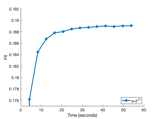
We now demonstrate how to plot the fit over time using info (the third output). The entry info.iters is the number of epochs performed by the algorithm, and the vectors info.time_trace and info.fit_trace contain the time and fit at the end of each epoch. The fit over time can then be plotted as shown in the example below.

% Plot the fit over time
figure(1)

hold on;
plot(info1.time_trace, info1.fit_trace, '-*','LineWidth', 3,...
    'Displayname', 's=2^{17}');
hold off;

legend('location', 'southeast')
ylim([0.175, 0.192]);

xlabel('Time (seconds)');
ylabel('Fit');
set(gca,'FontSize',14);

Specifying the number of samples

The number of fiber samples used for each least squares solve can be set via the argument nsamplsq. Decreasing the samples leads to faster iterations but can also result in lower fits. Generally s needs to be set via hyperparameter search but the default value (2^17) is typically an effective starting point. Set the next section for a discussion of how to set s.

% Run the algorithm:
rng("default"); % Set random seed for reproducibility
tic
[M, ~, info2] = cp_arls_lev(X,R,'truefit', 'iter', 'nsamplsq', 2^16);
time2 = toc;
fprintf('\n*** Results for CP-ARLS-LEV ***\n');
fprintf('Time (secs): %.3f\n', time2)
fprintf('Fit: %.3f\n', info2.finalfit)

Preprocessing Finished 

CP-ARLS with Leverage Score Sampling:

Tensor size: 183 x 24 x 1140 x 1717 (8596812960 total entries)
Sparse tensor: 3309490 (0.038%) Nonzeros and 8593503470 (99.96%) Zeros
Finding CP decomposition with R=25
Initialization: random (uniform)
Fit change tolerance: 1.00e-04
Epoch size: 5
Max epochs without improvement: 3
Max epochs overall: 50
Row samples per solve: 65536
No deterministic inclusion 
Fit based on: True residual
When to calculate true fit? iter

Iter  1x5: f = 1.780277e-01 f-delta =  2e-01 time = 3.5s (fit time = 1.1s) newi = 0
Iter  2x5: f = 1.833424e-01 f-delta =  5e-03 time = 3.4s (fit time = 1.1s) newi = 0
Iter  3x5: f = 1.849383e-01 f-delta =  2e-03 time = 3.4s (fit time = 1.1s) newi = 0
Iter  4x5: f = 1.858710e-01 f-delta =  9e-04 time = 3.4s (fit time = 1.1s) newi = 0
Iter  5x5: f = 1.867423e-01 f-delta =  9e-04 time = 3.5s (fit time = 1.1s) newi = 0
Iter  6x5: f = 1.872001e-01 f-delta =  5e-04 time = 3.3s (fit time = 1.1s) newi = 0
Iter  7x5: f = 1.876229e-01 f-delta =  4e-04 time = 3.3s (fit time = 1.1s) newi = 0
Iter  8x5: f = 1.876951e-01 f-delta =  7e-05 time = 3.4s (fit time = 1.1s) newi = 1
Iter  9x5: f = 1.878822e-01 f-delta =  3e-04 time = 3.2s (fit time = 1.1s) newi = 0
Iter 10x5: f = 1.880405e-01 f-delta =  2e-04 time = 3.1s (fit time = 1.1s) newi = 0
Iter 11x5: f = 1.881168e-01 f-delta =  8e-05 time = 3.2s (fit time = 1.1s) newi = 1
Iter 12x5: f = 1.880600e-01 f-delta =  2e-05 time = 3.1s (fit time = 1.1s) newi = 2
Iter 13x5: f = 1.880705e-01 f-delta =  3e-05 time = 3.3s (fit time = 1.1s) newi = 3

Final f = 1.880405e-01
Total time: 4.31e+01


*** Results for CP-ARLS-LEV ***
Time (secs): 43.076
Fit: 0.188

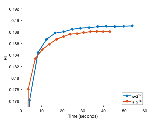
Plotting the resuts shows that for nsamplsq set to 2^16, the epochs are faster but the final fit is not as high as the default value of 2^17 because the accuracy of each least squares solve is lower.

% Plot the fit over time
figure(2)

hold on;
plot(info1.time_trace, info1.fit_trace, '-*','LineWidth', 3,...
    'Displayname', 's=2^{17}');
plot(info2.time_trace, info2.fit_trace, '-*','LineWidth', 3,...
    'Displayname', 's=2^{16}');
hold off;

legend('location', 'southeast')
ylim([0.175, 0.192]);

xlabel('Time (seconds)');
ylabel('Fit');
set(gca,'FontSize',14);

How to Select the Number of Samples

Theory for the number of samples required to obtain a solution whose residual is within $(1 \pm \epsilon)$ of the residual of the optimal solution with probability $1 - \delta$ can be found in Theorem 8 of the paper "Practical Leverage-Based Sampling for Low-Rank Tensor Decompositions." The theory guarantees this will occur for an order $d+1$ tensor if $s \geq r^d \max\left \{ C \log(r/\delta), 1/(\delta \epsilon)\right \}$ where $C = 144/(1 - 1/\sqrt{2})^2 \approx 1678.59$ . However, this bound is still pessimistic, as was shown in expeirments on the Uber tensor in Figure 3 of the paper. In our experiments, $s = 2^{17}$ provided sufficiently good performance whereas with $\delta = 0.01$ , $R = 25$ , and $\epsilon = 0.01$ the theory requires $s = 2^{23}$ . We thus advise that some hyperparameter search on $s$ may be necessary to ensure the right trade-off between accuracy and iteration time.

Comparing with CP-ALS

Here we compare the fit and timing of CP-ARLS-LEV to a single run of CP-ALS.

rng("default"); % Set random seed for reproducibility
tic;
M = cp_als(X,R,'printitn',10);
time_als = toc;
fprintf('Total Time (secs): %.3f\n', time_als)

% Compare runtime to CP-ARLS-LEV
diff = (time_als - time1);
fprintf('Extra time cost for CP-ALS: %.2f\n', diff)

CP_ALS:
 Iter 10: f = 1.826842e-01 f-delta = 7.9e-04
 Iter 20: f = 1.867754e-01 f-delta = 2.1e-04
 Iter 30: f = 1.881704e-01 f-delta = 1.2e-04
 Iter 37: f = 1.889253e-01 f-delta = 9.7e-05
 Final f = 1.889253e-01 
Total Time (secs): 242.920
Extra time cost for CP-ALS: 189.11

Running with estimated fit

For the Uber tensor and other tensors of this approximate size, calculating the true fit of the model tensor at the end of every epoch is a reasonable cost. However, for much larger tensors (e.g. those with the number of nonzeros in the hundred million or several billion), calcuting the true fit becomes prohibitive and will dominate the cost of the run. By passing 'iter' or 'never' as an option to truefit, we can specify that at the end of each epoch we want to approximate the fit based on a set of sampled elements. For sparse tensors, the method will default to stratified sampling with nsampfit nonzeros and nsampfit zeros. For dense tensors, the method will default to sampling 2*nsampfit elements of the tensor uniformly. Note that the elements are only drawn once to allow for better comparison of the estimated fit across iterations.

% Run the algorithm:
rng("default"); % Set random seed for reproducibility
tic
[M, ~, info3] = cp_arls_lev(X,R,'nsampfit', 2^19);
time = toc;

% Compute the final fit
normX = norm(X);
normresidual = sqrt( normX^2 + norm(M)^2 - 2 * innerprod(X,M) );
finalfit = 1 - (normresidual / normX); %Fraction explained by model

% Print run results
fprintf('\n*** Results for CP-ARLS-LEV ***\n');
fprintf('Time (secs): %.3f\n', time)
fprintf('Fit: %.3f\n', finalfit)

Preprocessing Finished 

CP-ARLS with Leverage Score Sampling:

Tensor size: 183 x 24 x 1140 x 1717 (8596812960 total entries)
Sparse tensor: 3309490 (0.038%) Nonzeros and 8593503470 (99.96%) Zeros
Finding CP decomposition with R=25
Initialization: random (uniform)
Fit change tolerance: 1.00e-04
Epoch size: 5
Max epochs without improvement: 3
Max epochs overall: 50
Row samples per solve: 131072
No deterministic inclusion 
Fit based on: stratified with 524288 nonzero and 524288 zero samples
When to calculate true fit? never

Iter  1x5: f~ = 1.655766e-01 f-delta =  2e-01 time = 2.8s (fit time = 0.1s) newi = 0
Iter  2x5: f~ = 1.774131e-01 f-delta =  1e-02 time = 2.9s (fit time = 0.1s) newi = 0
Iter  3x5: f~ = 1.809288e-01 f-delta =  4e-03 time = 3.9s (fit time = 0.1s) newi = 0
Iter  4x5: f~ = 1.806015e-01 f-delta = -3e-04 time = 3.3s (fit time = 0.1s) newi = 1
Iter  5x5: f~ = 1.834071e-01 f-delta =  2e-03 time = 3.1s (fit time = 0.1s) newi = 0
Iter  6x5: f~ = 1.821197e-01 f-delta = -1e-03 time = 3.2s (fit time = 0.1s) newi = 1
Iter  7x5: f~ = 1.827541e-01 f-delta = -7e-04 time = 3.0s (fit time = 0.1s) newi = 2
Iter  8x5: f~ = 1.840439e-01 f-delta =  6e-04 time = 3.0s (fit time = 0.1s) newi = 0
Iter  9x5: f~ = 1.819886e-01 f-delta = -2e-03 time = 3.2s (fit time = 0.1s) newi = 1
Iter 10x5: f~ = 1.836076e-01 f-delta = -4e-04 time = 4.7s (fit time = 0.1s) newi = 2
Iter 11x5: f~ = 1.815522e-01 f-delta = -2e-03 time = 3.5s (fit time = 0.1s) newi = 3

Final f~ = 1.840439e-01
Total time: 3.68e+01


*** Results for CP-ARLS-LEV ***
Time (secs): 36.768
Fit: 0.189

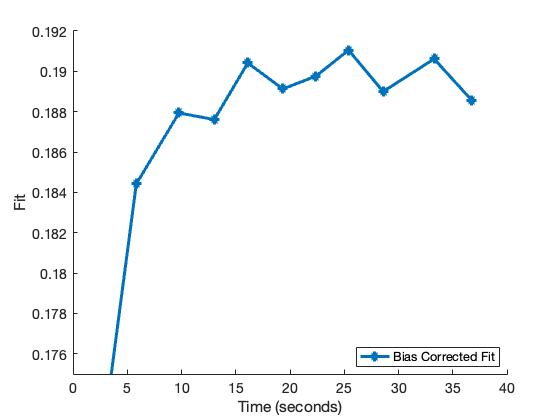
Because we are only drawing the elements once, this will result in the estimated fit being biased; it is recommended that results be bias corrected as demonstrated here.

% Compute the bias of the estimated fit and bias correct the results
bias = info3.fit_trace(end) - finalfit;
fprintf('Bias: %.3f\n', bias)
fit_trace_corrected = info3.fit_trace - bias;

% Plot the bias corrected results
figure(3)

hold on;
plot(info3.time_trace, fit_trace_corrected, '-*','LineWidth', 3,...
    'Displayname', 'Bias Corrected Fit');
hold off;

legend('location', 'southeast')
ylim([0.175, 0.192]);

xlabel('Time (seconds)');
ylabel('Fit');
set(gca,'FontSize',14);

Bias: -0.007

Running with hybrid sampling

During a run of CP-ARLS-LEV, the leverage scores can become very concentrated such that a small number of rows are repeatedly sampled. It can be helpful to instead to include these high leverage score rows deterministically before randomly sampling from the remaining rows. This can be done by specifying thresh which will result in all rows with a probability greater than this value being included in the sample deterministically. Note that this value should be set conservatively as the lower the threshold, the more time it will take in each iteration to identify the deterministically included rows. In general, we recommend one over the number of samples.

rng("default"); % Set random seed for reproducibility
s = 2^17;
tic
[M, ~, info] = cp_arls_lev(X,R,'truefit','iter','nsamplsq',s,'thresh',1.0/s);
time1 = toc;
fprintf('\n*** Results for CP-ARLS-LEV ***\n');
fprintf('Time (secs): %.3f\n', time1)
fprintf('Fit: %.3f\n', info.finalfit)

Preprocessing Finished 

CP-ARLS with Leverage Score Sampling:

Tensor size: 183 x 24 x 1140 x 1717 (8596812960 total entries)
Sparse tensor: 3309490 (0.038%) Nonzeros and 8593503470 (99.96%) Zeros
Finding CP decomposition with R=25
Initialization: random (uniform)
Fit change tolerance: 1.00e-04
Epoch size: 5
Max epochs without improvement: 3
Max epochs overall: 50
Row samples per solve: 131072
Threshold for deterministic sampling: 7.629395e-06
Fit based on: True residual
When to calculate true fit? iter

Iter  1x5: f = 1.774870e-01 f-delta =  2e-01 time = 7.3s (fit time = 1.0s) newi = 0
Iter  2x5: f = 1.837535e-01 f-delta =  6e-03 time = 7.4s (fit time = 1.1s) newi = 0
Iter  3x5: f = 1.863827e-01 f-delta =  3e-03 time = 6.8s (fit time = 1.1s) newi = 0
Iter  4x5: f = 1.875607e-01 f-delta =  1e-03 time = 7.1s (fit time = 1.1s) newi = 0
Iter  5x5: f = 1.879506e-01 f-delta =  4e-04 time = 7.9s (fit time = 1.1s) newi = 0
Iter  6x5: f = 1.880050e-01 f-delta =  5e-05 time = 6.9s (fit time = 1.2s) newi = 1
Iter  7x5: f = 1.885686e-01 f-delta =  6e-04 time = 6.5s (fit time = 1.0s) newi = 0
Iter  8x5: f = 1.888701e-01 f-delta =  3e-04 time = 6.6s (fit time = 1.1s) newi = 0
Iter  9x5: f = 1.890842e-01 f-delta =  2e-04 time = 7.1s (fit time = 1.0s) newi = 0
Iter 10x5: f = 1.891949e-01 f-delta =  1e-04 time = 6.8s (fit time = 1.0s) newi = 0
Iter 11x5: f = 1.892310e-01 f-delta =  4e-05 time = 6.6s (fit time = 1.0s) newi = 1
Iter 12x5: f = 1.894760e-01 f-delta =  3e-04 time = 6.6s (fit time = 1.0s) newi = 0
Iter 13x5: f = 1.895827e-01 f-delta =  1e-04 time = 6.6s (fit time = 1.0s) newi = 0
Iter 14x5: f = 1.897109e-01 f-delta =  1e-04 time = 6.5s (fit time = 1.0s) newi = 0
Iter 15x5: f = 1.897940e-01 f-delta =  8e-05 time = 6.5s (fit time = 1.0s) newi = 1
Iter 16x5: f = 1.898870e-01 f-delta =  2e-04 time = 6.5s (fit time = 1.0s) newi = 0
Iter 17x5: f = 1.897943e-01 f-delta = -9e-05 time = 6.6s (fit time = 1.0s) newi = 1
Iter 18x5: f = 1.899749e-01 f-delta =  9e-05 time = 6.8s (fit time = 1.0s) newi = 2
Iter 19x5: f = 1.899726e-01 f-delta =  9e-05 time = 6.4s (fit time = 1.0s) newi = 3

Final f = 1.898870e-01
Total time: 1.30e+02


*** Results for CP-ARLS-LEV ***
Time (secs): 129.617
Fit: 0.190

What is contained in the output info

The third output, which we usually call info, contains information about the run. This output has the following fields:

params: Contains the input parameters for the run
truefit: The setting for the input parameter truefit
preproc_time: Timing for various parts of preprocessing (1. Extract tensor properties, 2. Parse parameters, 3. Get fiber indices for each mode, sparse tensors only, 4. Set up random initialization, 5. Compute initial leverage scores)
iters: Number of epochs for the run
finalfit: Final fit, will be NaN if truefit is set to 'never'
time_trace: Time at the end of each epoch
fit_trace: Fit at the end of each epoch
normresidual_trace: Norm residual at the end of each epoch
total_time: Total time for the run, including preprocessing and final fit computation if included